How to Add Watermark in Excel on PC or Mac

Open your spreadsheet in Microsoft Excel. You can usually do this by double-clicking the file on your computer.

Click the Insert tab. It’s on the left side of the tab bar at the top of Excel.

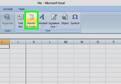
Click Header & Footer. It’s near the end of the row of icons at the top of Excel. Its icon looks like a white sheet of paper with orange markings at its top and bottom edges.

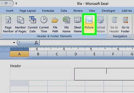
Click Picture. It’s in the group of icons labeled “Header & Footer elements" at the top of Excel, near the center.

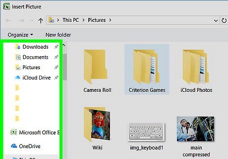
Click Browse. It’s next to “From a file.” This opens the file browser.

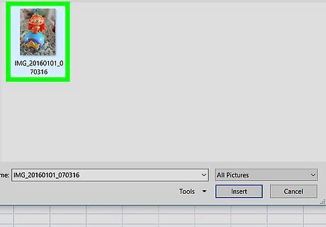
Click the image you want to use as a watermark. This is usually a logo, name, or a text warning.

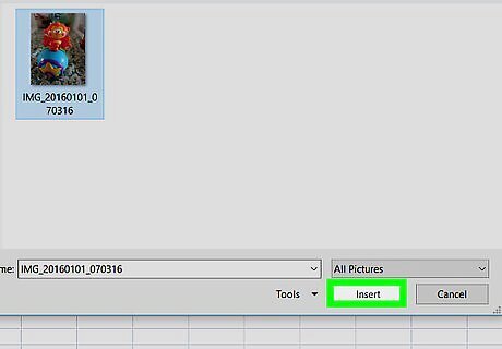
Click Insert. This overlays the image on your spreadsheet.

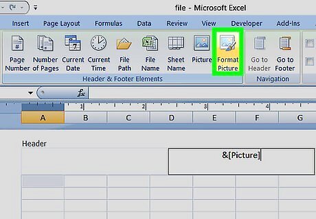
Click Format Picture. It’s the photo icon in the “Header & Footer Elements” group at the top of Excel. This opens the "Format Picture" window to the “Size” tab.

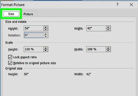
Adjust the size of the watermark. Use the drop-down menus on the “Size” tab set the height and width of the watermark.

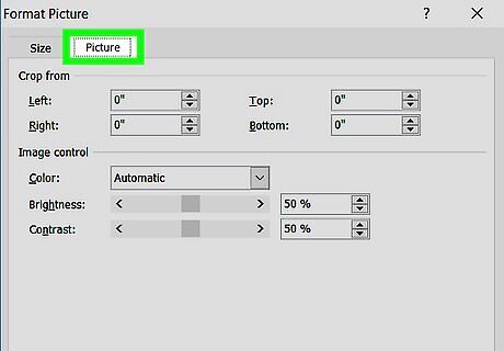
Click the Picture tab. It’s at the top of the "Format Picture" window.

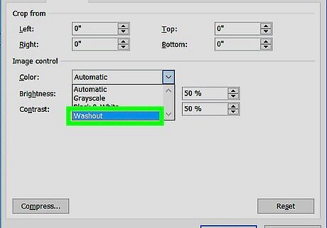
Select Washout from the “Color” drop-down. It’s under the “Image control” header. This fades the watermark so that it doesn’t completely block out the content of the spreadsheet. It’ll still be visible, just less opaque.

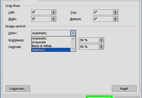
Click OK. This returns you to the spreadsheet and your newly-formatted watermark. Click anywhere on the spreadsheet to return to regular editing mode.