
Enabling Gridlines (Windows)

Open a worksheet in Microsoft Excel. You can use an existing project or create a new spreadsheet. Gridlines can't be customized in the same way borders can. For more customization options with cell borders, see this section.
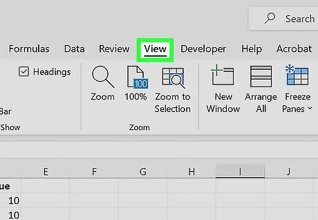
Click View. This is the tab at the top.
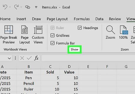
Locate the "Show" section. This will be between the Workbook Views and Zoom section. You should see a list of options, such as Ruler, Gridlines, Formula Bar, etc.
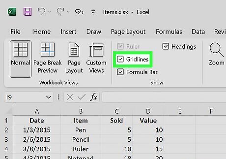
Check the box next to "Gridlines". When this box is checked, you'll see the gridlines appear on your Excel worksheet. Gridlines do not print by default. If you want to print with the gridlines on, do the following: Click the Page layout tab at the top. Find the Sheet Options section. Check the box next to Print underneath Gridlines.
Enabling Gridlines (Mac)
Open a worksheet in Microsoft Excel. You can use an existing project or create a new spreadsheet.
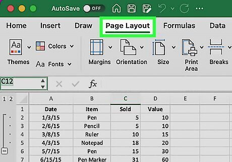
Click Page Layout. This is in the top toolbar.
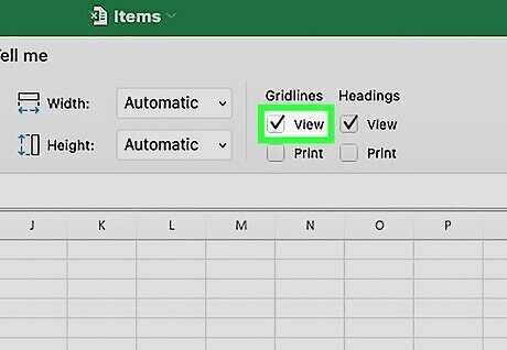
Check the "View" box. This will be underneath Gridlines. When this box is checked, you'll see the gridlines appear on your Excel worksheet. If you want to print with the gridlines on, check the box next to Print.
Adding Cell Borders
Open a worksheet in Microsoft Excel. You can use an existing project or create a new spreadsheet. Gridlines appear on all sheets by default, but they may not be bold enough to make your data stand out. If you want to surround certain data with more visible lines, you can add borders to those cells.
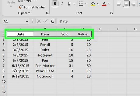
Select the range of cells you want to add borders to. You will be able to add a border that surrounds the entire selected range, and/or around each individual cell in the range.
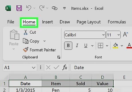
Click the Home tab. It's at the top of Excel.

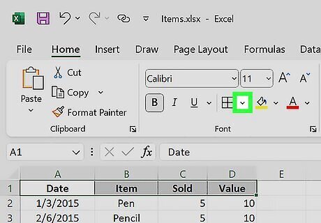
Click the arrow next to the Borders icon. The Borders icon is a dotted grid on the "Font" panel at the top of Excel. A list of border styles will appear.
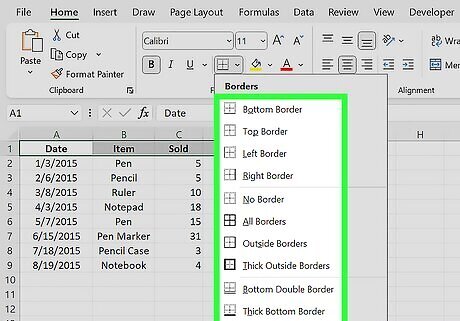
Select a border style. If you want to add darker grid lines that surround each selected cell, choose All Borders. Otherwise, choose any of the other options, such as Outside Borders, which adds one solid border around the selected range.
Click the arrow next to the "Borders" icon again. Now that you've inserted some cell borders, you can customize how they look.
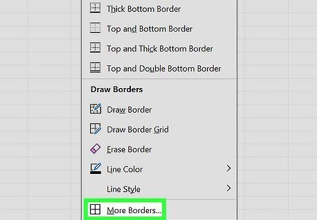
Click More Borders…. It's at the bottom of the menu.
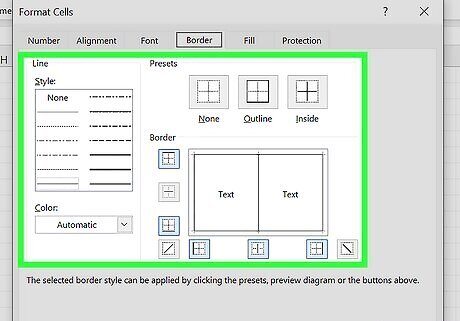
Choose your border options. You can customize the line style, border style, and even color. To customize the actual line used in the border (such as changing a solid line to a dotted line), select one of the line styles from the Styles area. To make the border a different color, choose a color from the Color menu.
Click OK. This adds your border preferences to the selected range. To remove cell borders, click the arrow next to the Borders icon in the toolbar, and then choose No Border. Unlike gridlines, cell borders are always shown on printed sheets.


Comments
0 comment